Chapter 2 Basic Computer Architecture
2.1 Typical Machine Layout
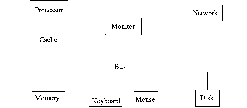
Figure based on M. L. Scott, Programming Language Pragmatics, Figure 5.1, p. 205
2.2 Structure of Lab Workstations
2.2.1 Processor and Cache
luke@l-lnx200 ~% lscpu
Architecture:            x86_64
  CPU op-mode(s):        32-bit, 64-bit
  Address sizes:         46 bits physical, 48 bits virtual
  Byte Order:            Little Endian
CPU(s):                  24
  On-line CPU(s) list:   0-23
Vendor ID:               GenuineIntel
  Model name:            12th Gen Intel(R) Core(TM) i9-12900K
    CPU family:          6
    Model:               151
    Thread(s) per core:  2
    Core(s) per socket:  16
    Socket(s):           1
    Stepping:            2
    CPU(s) scaling MHz:  59%
    CPU max MHz:         5200.0000
    CPU min MHz:         800.0000
    BogoMIPS:            6374.40
    Flags:               ...
Virtualization features:
  Virtualization:        VT-x
Caches (sum of all):
  L1d:                   640 KiB (16 instances)
  L1i:                   768 KiB (16 instances)
  L2:                    14 MiB (10 instances)
  L3:                    30 MiB (1 instance)
...
There is a single 16-core processor with hyperthreading that acts like 24 separate processors
Hyperthreading is enabled, which makes each core to some extent behave like two processors.
The total L3 cache is 30MiB
2.2.2 Memory and Swap Space
luke@l-lnx200 ~% free -m
               total        used        free      shared  buff/cache   available
Mem:           31924        1144       20258          25       10521       30258
Swap: 24255 0 24255- The workstations have about 32G of memory.
- The swap space is about 24G.
2.2.3 Disk Space
Using the df command produces:
luke@l-lnx200 ~% df -BG
Filesystem                1G-blocks  Used Available Use% Mounted on
...
/dev/nvme0n1p2                   1G    1G        1G  16% /boot
/dev/mapper/vg00-tmp             8G    1G        8G   1% /tmp
/dev/mapper/vg00-var            47G   15G       31G  33% /var
...
/dev/mapper/vg00-scratch        26G    1G       26G   1% /var/scratch
...
clasnetappvm...:/students      300G  144G      157G  48% /mnt/nfs/clasnetappvm/students
...
clasnetappvm...:/shared         82G   20G       63G  24% /mnt/nfs/clasnetappvm/shared
...
clasnetappvm...:/grad         1536G  560G      977G  37% /mnt/nfs/clasnetappvm/grad
...
Local disks are large but mostly unused
Space in
/var/scratchcan be used for temporary storage.User space is on network disks.
Network speed can be a bottle neck.
2.2.4 Performance Monitoring
Using the top command produces:
top - 11:06:34 up  4:06,  1 user,  load average: 0.00, 0.01, 0.05
Tasks: 127 total,   1 running, 126 sleeping,   0 stopped,   0 zombie
Cpu(s):  0.0%us,  0.0%sy,  0.0%ni, 99.8%id,  0.2%wa,  0.0%hi,  0.0%si,  0.0%st
Mem:  16393524k total,   898048k used, 15495476k free,   268200k buffers
Swap: 18481148k total,        0k used, 18481148k free,   217412k cached

  PID USER      PR  NI  VIRT  RES  SHR S %CPU %MEM    TIME+  COMMAND
 1445 root      20   0  445m  59m  23m S  2.0  0.4   0:11.48 kdm_greet
    1 root      20   0 39544 4680 2036 S  0.0  0.0   0:01.01 systemd
    2 root      20   0     0    0    0 S  0.0  0.0   0:00.00 kthreadd
    3 root      20   0     0    0    0 S  0.0  0.0   0:00.00 ksoftirqd/0
    5 root       0 -20     0    0    0 S  0.0  0.0   0:00.00 kworker/0:0H
    6 root      20   0     0    0    0 S  0.0  0.0   0:00.00 kworker/u:0
    7 root       0 -20     0    0    0 S  0.0  0.0   0:00.00 kworker/u:0H
    8 root      RT   0     0    0    0 S  0.0  0.0   0:00.00 migration/0
    9 root      RT   0     0    0    0 S  0.0  0.0   0:00.07 watchdog/0
   10 root      RT   0     0    0    0 S  0.0  0.0   0:00.00 migration/1
   12 root       0 -20     0    0    0 S  0.0  0.0   0:00.00 kworker/1:0H
   13 root      20   0     0    0    0 S  0.0  0.0   0:00.00 ksoftirqd/1
   14 root      RT   0     0    0    0 S  0.0  0.0   0:00.10 watchdog/1
   15 root      RT   0     0    0    0 S  0.0  0.0   0:00.00 migration/2
   17 root       0 -20     0    0    0 S  0.0  0.0   0:00.00 kworker/2:0H
   18 root      20   0     0    0    0 S  0.0  0.0   0:00.00 ksoftirqd/2
   ...
Interactive options allow you to kill or renice (change the priority of) processes you own.
The command
htopmay be a little nicer to work with.A GUI tool,
System Monitor, is available from one of the menus. From the command line this can be run asgnome-system-monitor.
Another useful command is ps (process status)
luke@l-lnx200 ~% ps -u luke
  PID TTY          TIME CMD
 4618 ?        00:00:00 sshd
 4620 pts/0    00:00:00 tcsh
 4651 pts/0    00:00:00 ps
There are many options; see man ps for details.
2.3 Processors
2.3.1 Basics
Processors execute a sequence of instructions.
Each instruction requires some of
- decoding instruction
- fetching operands from memory
- performing an operation (add, multiply, …)
- etc.
Older processors would carry out one of these steps per clock cycle and then move to the next.
Most modern processors use pipelining to carry out some operations in parallel.
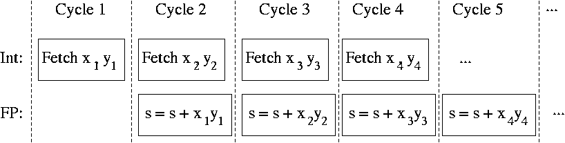
2.3.2 Pipelining
A simple example:
for \(i = 1\) to \(n\) do
\(s \leftarrow s + x_i y_i\)
end
Simplified view: Each step has two parts,
- Fetch \(x_i\) and \(y_i\) from memory
- Compute \(s = s + x_i y_i\)
Suppose the computer has two functional units that can operate in parallel,
- An Integer unit that can fetch from memory
- A Floating Point unit that can add and multiply
If each step takes roughly the same amount of time, a pipeline can speed the computation by a factor of two:
Floating point operations are much slower than this.
Modern chips contain many more separate functional units.
Pipelines can have 10 or more stages.
Some operations take more than one clock cycle.
The compiler or the processor orders operations to keep the pipeline busy.
If this fails, then the pipeline stalls.
2.3.3 Superscalar Processors, Hyper-Threading, and Multiple Cores
Some processors have enough functional units to have more than one pipeline running in parallel.
Such processors are called superscalar.
In some cases there are enough functional units per processor to allow one physical processor to pretend like it is two (somewhat simpler) logical processors. This approach is called hyper-threading.
Hyper-threaded processors on a single physical chip share some resources, in particular cache.
Benchmarks suggest that hyper-threading produces about a 20% speed-up in cases where dual physical processors would produce a factor of 2 speed-up
It is now possible to fully replicate processors within one chip; these are multi core processors.
Multi-core machines are effectively full multi-processor machines (at least for most purposes).
Dual core processors are now ubiquitous.
The department research machine
r-lnx404has two 16-core processors.Our lab machines have a single 16-core processor.
Processors with even more cores are available.
Many processors support some form of vectorized operations, e.g. SSE2 (Single Instruction, Multiple Data, Extensions 2) on Intel and AMD processors.
GPUs provide even more parallelism but require specialized programming.
2.3.4 Implications
Modern processors achieve high speed though a collection of clever tricks.
Most of the time these tricks work extremely well.
Every so often a small change in code may cause pipelining heuristics to fail, resulting in a pipeline stall.
These small changes can then cause large differences in performance.
The chances are that a “small change” in code that causes a large change in performance was not in fact such a small change after all.
Processor speeds have not been increasing very much recently.
Though the arm64 family (Apple M1) has produced some significant
speedups while reducing power consumption.
Many believe that speed improvements will need to come from increased use of explicit parallel programming.
More details are available in a talk at
https://www.infoq.com/presentations/click-crash-course-modern-hardware/
2.4 Memory
2.4.1 Basics
Data and program code are stored in memory.
Memory consists of bits (binary integers)
On most computers
Bits are collected into groups of eight, called a byte.
There is a natural word size of \(W\) bits.
The most common value of \(W\) used to be 32; it is probably now 64; 16 also occurs.
Bytes are numbered consecutively, \(0, 1, 2, \dots, N = 2^W\).
An address for code or data is a number between \(0\) and \(N\) representing a location in memory, usually in bytes.
\(2^{32} = 4,294,967,296 = 4\text{GB}\).
The maximum amount of memory a 32-bit process can address is 4 Gigabytes.
Some 32-bit machines can use more than 4G of memory, but each process gets at most 4G.
Most hard disks are much larger than 4G.
2.4.2 Memory Layout
A process can conceptually access up to \(2^W\) bytes of address space.
The operating system usually reserves some of the address space for things it does on behalf of the process.
On 32-bit Linux the upper 1GB is reserved for the operating system kernel.
Only a portion of the usable address space has memory allocated to it.
Standard 32-bit Linux memory layout:

The standard heap can only grow to 1G.
malloc implementations can allocate more using memory mapping.
Obtaining large amounts of contiguous address space can be hard.
Memory allocation can slow down when memory mapping is needed.
Other operating systems differ in detail only.
64-bit machines are much less limited.
The design matrix for \(n\) cases and \(p\) variables stored in double precision needs \(8np\) bytes of memory.
| \(p = 10\) | \(p = 100\) | \(p = 1000\) | |
|---|---|---|---|
| n = 100 | 8,000 | 80,000 | 800,000 |
| n = 1,000 | 80,000 | 800,000 | 8,000,000 |
| n = 10,000 | 800,000 | 8,000,000 | 80,000,000 |
| n = 100,000 | 8,000,000 | 80,000,000 | 800,000,000 |
2.4.3 Virtual and Physical Memory
To use address space, a process must ask the kernel to map physical space to the address space.
There is a hierarchy of physical memory:
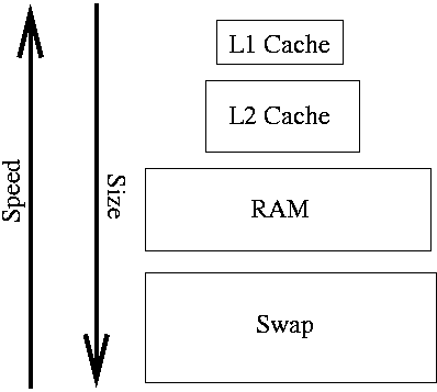
Hardware/OS hides the distinction.
Caches are usually on or very near the processor chip and very fast.
RAM usually needs to be accessed via the bus
The hardware/OS try to keep recently accessed memory and locations nearby in cache.
A simple example:
msum <- function(x) {
    nr <- nrow(x)
    nc <- ncol(x)
    s <- 0
    for (i in 1 : nr)
        for (j in 1 : nc)
            s <- s + x[i, j]
    s
}
m <- matrix(0, nrow = 5000000, 2)
system.time(msum(m))
##   user  system elapsed
## 1.712 0.000 1.712 fix(msum) ## reverse the order of the sums
system.time(msum(m))
## user system elapsed
## 0.836 0.000 0.835 Matrices are stored in column major order.
This effect is more pronounced in low level code.
Careful code tries to preserve locality of reference.
2.4.4 Registers
Registers are storage locations on the processor that can be accessed very fast.
Most basic processor operations operate on registers.
Most processors have separate sets of registers for integer and floating point data.
On some processors, including i386 and x64, the floating point registers have extended precision.
Optimizing compilers work hard to keep data in registers.
Small code changes can cause dramatic speed changes in optimized code because they make it easier or harder for the compiler to keep data in registers.
If enough registers are available, then some function arguments can be passed in registers.
Vector support facilities, like SSE2, provide additional registers that compilers may use to improve performance.
2.5 Processes and Shells
A shell is a command line interface to the computer’s operating system.
Common shells on Linux and MacOS are bash and tcsh.
You can now set your default Linix shell at https://hawkid.uiowa.edu/.
Shells are used to interact with the file system and to start processes that run programs.
You can set process limits and environment variables in the shell.
Programs run from shells take command line arguments.
2.5.1 Some Basic bash/tcsh Commands
hostname prints the name of the computer the shell is running on.
pwd prints the current working directory.
ls lists files a directory
lslists files in the current directory.ls foolists files in a sub-directoryfoo.
cd changes the working directory:
cdorcd ~moves to your home directory;cd foomoves to the sub-directoryfoo;cd ..moves up to the parent directory;
mkdir foo creates a new sub-directory foo in your current working
directory;
rm, rmdir can be used to remove files and directories; BE VERY
CAREFUL WITH THESE!!!
2.5.2 Standard Input, Standard Output, and Pipes
Programs can also be designed to read from standard input and write to standard output.
Shells can redirect standard input and standard output.
Shells can also connect processes into pipelines.
On multi-core systems pipelines can run in parallel.
A simple example using the bash shell script
P1.sh:
#!/bin/bash

while true; do echo $1; done
This can be run using the rev program as
bash P1.sh fox
bash P1.sh fox > /dev/null
bash P1.sh fox | rev
bash P1.sh fox | rev > /dev/null
bash P1.sh fox | rev | rev > /dev/null
Examples are available here.