Determining effect sizes--Fixed effects

 The dialogs focus on the power of an F test, which in turn depends (among other things) on the effect size corresponding to some alternative hypothesis of interest. We quantify effect size to be the standard deviation of the effects in the ANOVA model; this choice is made for two reasons:

• It has a meaningful interpretation for fixed, random, and mixed effects.
• It has the same units of measurement (centimeters, seconds, etc.) as the data.

In spite of these advantages, there is also some potential confusion, as is warned earlier in this document.

An example

 To illustrate the underlying ideas, consider a two-way completely randomized factorial design. Specifically, following an example in Kuehl (1994), page 164, suppose that we wish to do an experiment to study the effects of aggregate type and kneading on the tensile strength of asphaltic concrete. The factors and levels are

Aggregate type Basalt, Silicious

Kneading Static, Regular, Low, Very low

and the response variable is tensile strength, in pounds per square inch (psi).

To determine effect sizes, we have to talk about goals for the experiment. In this case, we might consider anything less than a 10% difference to be fairly negligible, so a reasonable goal might be to be able to detect a 10% difference between two means with reasonable power. Supposing that we know from experience that the tensile strength will be in the range of 80 psi, then this goal translates to a difference of about 8 psi.

Main effects

For Aggregate Type, then, we would want to have the capability of detecting a difference if, hypothetically, the mean strengths are 76 psi and 84 psi (or vice versa). To get the corresponding effect size, first subtract the overall mean (thus obtaining -4 and +4); these represent the hypothetical effects of aggregate type. The effect SD to enter in the dialog is defined as

$$\mbox{Effect SD} = \sqrt{\sum (\mbox{effects})^2 / \mbox{(degrees of freedom)}}$$ (1)

 So the desired effect SD for aggregate type is $\sqrt{((-4)^2+4^2)/1} = \sqrt{32} \approx 5.66$ psi.

The thinking is a little more complicated when determining an effect size for Kneading. Supposing that we still want to detect differences of 8 psi or so between two means, there are several different corresponding scenarios. The effects could be {-4,+4,0,0}, or {-4,-4,+4,+4}, or {-4,-2,+2,+4}, or a variety of other possibilities (again, the order of these effects is unimportant). Noting that this four-level factor has 3 degrees of freedom and applying Equation (3.2), the corresponding effect SDs are $\sqrt{32/3} \approx 3.27, \sqrt{64/3}\approx4.62, \sqrt{40/3}\approx3.65$, respectively. It can be shown that the first two values are the minimum and maximum possible values, representing worst- and best-case scenarios. We might want to try all three of these effect SDs in the dialog to see what the range of power is.

Interaction effect

Now, consider the interaction. Perhaps you do not want to have any goals at all for the interaction, in which case you can just ignore it. Otherwise, it may be useful to think in terms of ``simple effects,'' i.e., comparisons within a row or column. Here are two scenarios of interaction effects for the concrete example:

These represent the worst and best-case scenarios, respectively, when some simple comparisons are as large as 8 psi. Note that every row and every column of each table sums to 0; otherwise, main effects would be in force and we would not have pure interaction effects. The effect SDs are again calculated using Equation (3.2), noting that the interaction has $1\times3=3$ degrees of freedom: $$\begin{eqnarray*} \mbox{Worst case:~~effect SD} &=& \sqrt{(4\times4^2)/3} = 4.62\ \mbox{Best case:~~~effect SD} &=& \sqrt{(8\times4^2)/3} = 6.53\ \end{eqnarray*}$$

The Effect Advisor

We recognize that the above methods are somewhat tedious. To aid in obtaining effect sizes for fixed effects and their interactions, an Effect Advisor application is available via the Options menu. 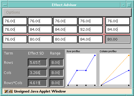It opens with a dialog where you choose the number of rows and columns to study; then, after clicking on ``OK'', the window is redrawn with data-entry fields for hypothetical cell means, marginal means, effect SDs, and effect ranges. The Effect Advisor dialog for our example (2 rows, 4 columns), looks like this:

 

If you change the value in any field and hit Enter or click elsewhere, all the other fields are updated appropriately. In addition, there are items in the Options menu to choose minimum-SD, maximum-SD, or linear effects (holding the range fixed) for rows, columns, and interaction. The above illustration was obtained by selecting minimum SDs for each term, setting all the ranges to 8.00, and setting the grand mean to 80. Note that the effect SDs shown are consistent with the minimum SDs obtained above. The interaction plots give a visual idea of these target effects.

The Effect Advisor is only set up for two factors. You can study more factors by working with two of them at a time (but there is no provision for interactions of higher order than 2). To study just one factor, just ignore either rows or columns and work with the marginal means of one factor.

Experimental error

Power cannot be determined without knowledge of the SD of the experimental error (and in general, the SDs of all sources of random error). Often, information about experimental error is estimated from a pilot study, or from past experiments with perhaps a different design but the same response variable and same structure of replications.

In the concrete example, suppose that we already have several specimens of concrete in the laboratory, all made from different batches but with the same ``recipe'' and kneading method. Thus, it is thought that the variations in tensile strength of these specimens are reasonably representative of the within-cell variations we can expect in the planned experiment. Seven of these specimens are tested, and we find that the sample variance is 12.50 (so that the SD is 3.54).

We may use 3.54 as an estimate of the within-cell SD in the power analysis. This is only an estimate; the true SD may be larger or smaller than this. When estimates are used (i.e., essentially always), the powers of tests are only estimates of the true powers. Power analysis is not an exact science, but it is a way of finding a reasonable sample size relative to the goals of a study.

Putting it together

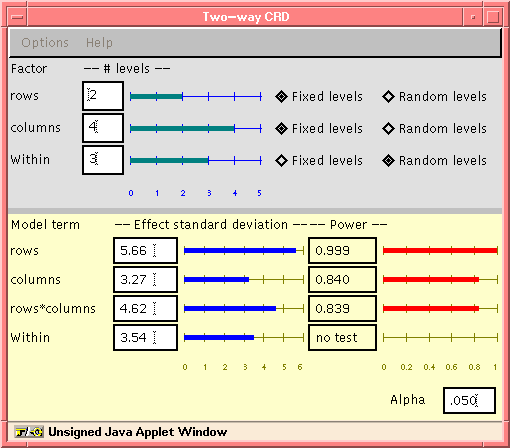
Now it's time to run the Java applet for planning the experiment. The dialog is shown below with the effect sizes computed above entered (the worst-case effect SDs are used for the Kneading and interaction terms). We also have to enter the correct numbers of levels for Aggregate type (``row''in the dialog) and Kneading (``column'' in the dialog).

 

The idea of determining sample size is to manipulate it and observe the powers of the tests of interest until acceptable results are achieved. At the .05 significance level (the default), a sample size of 3 observations per cell is sufficient to provide power exceeding 80% for all three goal values. (Note that sample size is inputted as the number of levels for ``Within.'') We therefore recommend that an experiment with 3 observations per cell (24 observations total) be conducted. The list of 24 factor combinations (3 copies of each) is arranged in random order to determine the protocol for a completely randomized experiment.

Incidentally, a power of 75-80% is often used as a target; a lower power than that does not provide a good chance of detecting the stated effect, and powers of 95% and higher usually require about twice as much data--wasting time, money, resources, and experimental animals' lives.

Do try this at home

 It is instructive to try out some variatioins on this example. Using a Java-capable web browser, connect to http://www.stat.uiowa.edu/~rlenth/Power/TwoWay.html . Here are some things to try:

1.

Reproduce the results above.

2.

What happens to the powers of the tests if the sample size is reduced to 2 observations per cell? Increased to 4?

3.

What happens if you change alpha to .01?

4.

What effect SD for rows can be detected with a power of .80? (Suggestion: drag on the effect-SD bar and watch the power bar.) What difference of means has this effect SD? (You'll have to do some math.) Often, the sample size is essentially determined by the budget, and such manipulations give us a measure of the capability of the experiment.

5.

Use the options menu, obtain a report of the current state of the power analysis.