Next: Assignment 5
Up: 22S:194 Statistical Inference II
Previous: Assignment 4
- 7.44
-
 are
are 
 .
.
 has
has
Since
 is sufficient and complete,
  is the UMVUE of
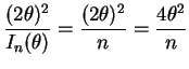
 . The CRLB is
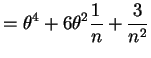
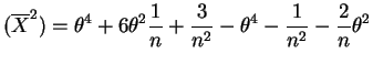
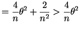
Now
So
- 7.48
- a.
- The MLE
 has variance
Var
has variance
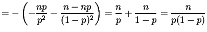
Var . The information is
So the CRLB is
 .
.
- b.
-
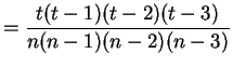
![$ E[X_{1}X_{2}X_{3}X_{4}]=p^{4}$](img226.png) .
.
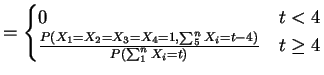
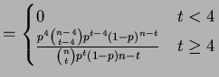
 is
sufficient and complete.
is
sufficient and complete.
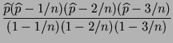
So the UMVUE is (for  )
)
No unbiased estimator eists for  .
.
- 7.62
- a.
-
- b.
- For
 ,
,
So
- c.
-
- 7.63
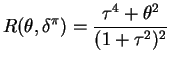
- From the previous problem, when the prior mean is zero the risk of
the Bayes rule is
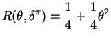
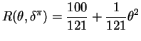
So for

and for

With a smaller  the risk is lower near the prior mean and
higher far from the prior mean.
the risk is lower near the prior mean and
higher far from the prior mean.
- 7.64
- For any
The independence assumptions imply that
 is
independent of
is
independent of
 and therefore.
for each  . Since
 is a Bayes rule for estimating
 with loss
 we have
with the final equality again following from the independence
assumptions. So
and therefore
for all  , which implies that
 is a
Bayes rule for estimating
is a
Bayes rule for estimating
 with
loss
with
loss
 and prior
 .
.
Next: Assignment 5
Up: 22S:194 Statistical Inference II
Previous: Assignment 4
Luke Tierney
2003-05-04
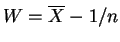
![$\displaystyle E[W] = \theta^{2}+\frac{1}{n}-\frac{1}{n} = \theta^{2}$](img207.png)

![$\displaystyle = \theta^{4}+4\theta^{3}\frac{1}{\sqrt{n}}E[Z] + 6\theta^{2}\frac{1}{n}E[Z^{2}]+4\theta\frac{1}{n^{3/2}}E[Z^{3}] + \frac{1}{n^{2}}E[Z^{4}]$](img214.png)
![$\displaystyle = -E\left[\frac{\partial^{2}}{\partial\theta^{2}} \left(\sum X_{i}\log p + \left(n-\sum X_{i}\right)\log(1-p)\right)\right]$](img222.png)
![$\displaystyle = -E\left[\frac{\partial}{\partial\theta}\left(\frac{\sum X_{i}}{p}-\frac{n-\sum X_{i}}{1-p}\right)\right]$](img223.png)
![$\displaystyle (\theta\vert X)] = E\left[\frac{\sigma^{2}\tau^{2}}{\sigma^{2}+n\tau^{2}}\right] = \frac{\sigma^{2}\tau^{2}}{\sigma^{2}+n\tau^{2}} = \eta\tau^{2}$](img250.png)