Problem: Let
 be constants, and
suppose
be constants, and
suppose
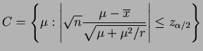
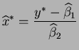
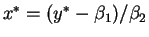
Let  be a constant and let let
  satisfy
that is, is the value of  at which the mean response is .
- a.
- Find the maximum likelihood estimator
 of .
of .
- b.
- Use the delta method to find the approximate sampling
distribution of
.
Solution: This prolem should have explicitly assumed normal
errors.
- a.
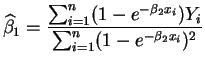
- Since
 , the MLE is
by MLE invariance.
- b.
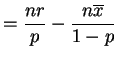
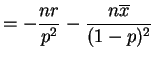
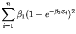
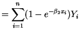
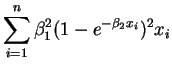
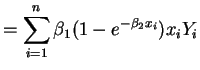
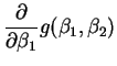
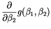
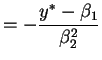
- The partial derivatives of the function
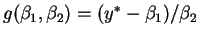 are
are
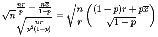
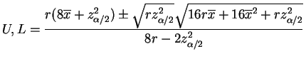
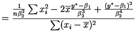
So for
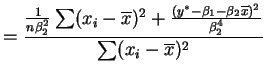
 the variance of the approximate sampling
distribution is
the variance of the approximate sampling
distribution is
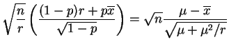
So by the delta method
 AN
AN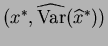 . The approximation is reasonably good if
 is far from zero, but the actual mean and variance of
do not exist.
is far from zero, but the actual mean and variance of
do not exist.